An Example of Linear Modeling in R

I. Introduction

Flight delays can be extremely frustrating, especially given the difficulty that consumers can face when trying to predict what factors might make a flight more or less delayed. Being able to predict how late a flight is based on a set of controllable factors would be extremely valuable. Hence, in this project we will attempt to create a model to predict flight delays, using a set of variables that could realistically be controlled by a prospective consumer.

We will be using the variables Month, Day, Day of the Week, Airline, Origin, Destination, Distance, Scheduled Departure. While this set contains observations from airports across the country, it does not seem reasonable to assume that a consumer could leave from any airport that they wanted. Hence, we will be using a subset of our original data set containing only flights from Oakland, San Francisco, and San Jose. While this limits the predictive power for non-Bay Area fliers, we hope that a similar model could be created to suit the needs of passengers leaving from other locations. Moreover, we will not be using all of the variables in our data set, instead opting to begin by modeling using the month, the day of the week, the airline being flown with, the origin airport (OAK, SFO, or SJC), the destination airport, the scheduled departure (in 24 hour time), and the distance being flown. Our thinking is that these are all variables that could be reasonably controlled by a consumer when choosing a flight.

Since our end-user is a traveler and not a government agency, only a subset of all the variables in our dataset is relevant to answering our research question. A is deciding where to book their ticket and from which airline to do so. They do not have access to information such as actual arrival times, taxi times, reasons for the delay, and other variables like such. A typical user will not have the ability nor the reason to consider these exogenous variables. Taxi time for example is a factor of how busy an airport is, how many planes are allowed in the sky at one time, the season, the weather, the economy, the number of operating airlines, proximity to a city, and various other factors that someone booking a trip will not go through the extreme research lengths to make a decision.

By regressing on the airport (both the destination and departure), we are implicitly able to capture these generalized variables. Likewise, variations in season and holidays are also implicitly captured by Month, Day, and Day of the week since our dataset is restricted to a single year.

Our report will be structured as follows. Section II will be devoted to a brief discussion of the data, its distributions, its limitations, and some transformations we will be applying to it. Section III will discuss our model, and how we came to it. Section IV will be devoted to testing our model and discussing our overall results. Finally, section V will be our conclusion, where we will discuss the results of this testing and possible next steps.

II. Data Description

Our data is provided by the U.S. Department of Transportation (DOT). The DOT Bureau of Transportation Statistics tracks the on-time performance of domestic flights operated by large air carriers. Summary information on the number of on-time, delayed, canceled, and diverted flights are published in the DOT’s monthly Air Travel Consumer Report where this dataset of 2015 flight delays and cancellations is sourced. The original dataset contains nearly 6 million observations. While this may prove useful about establishing trends about airline on-time performance nationally, for the focus of this project we will only consider flights originating from the 3 major airports of the Bay Area: San Francisco International Airport (SFO), Oakland International Airport (OAK), and Norman Y. Mineta San Jose International Airport (SJC).

III. Data Cleaning and Preprocessing

After extracting all the flight data from SFO, OAK, and SJO, we noticed that there are rows with missing values. This could potentially be the result of human error or data discrepancies across different airports or airlines. To mitigate this issue of regressing on missing values, we took the step of removing all rows with null or missing values. We then removed all the flights that are canceled since a canceled flight should not be part of the model predicting arrival delays. Lastly, we one-hot encoded all of our categorical variables from the last section, creating dummy variables for each airline, month, and day of the week.

Additionally, while this is technically data modification, it was in this step that we discovered that for whatever reason the DOT data that we acquired did not have correct departure airports for October (they were all given in the form of 5 digit numbers that we could not link to any airports). For that reason, October is not included in our analysis.

IV. EDA

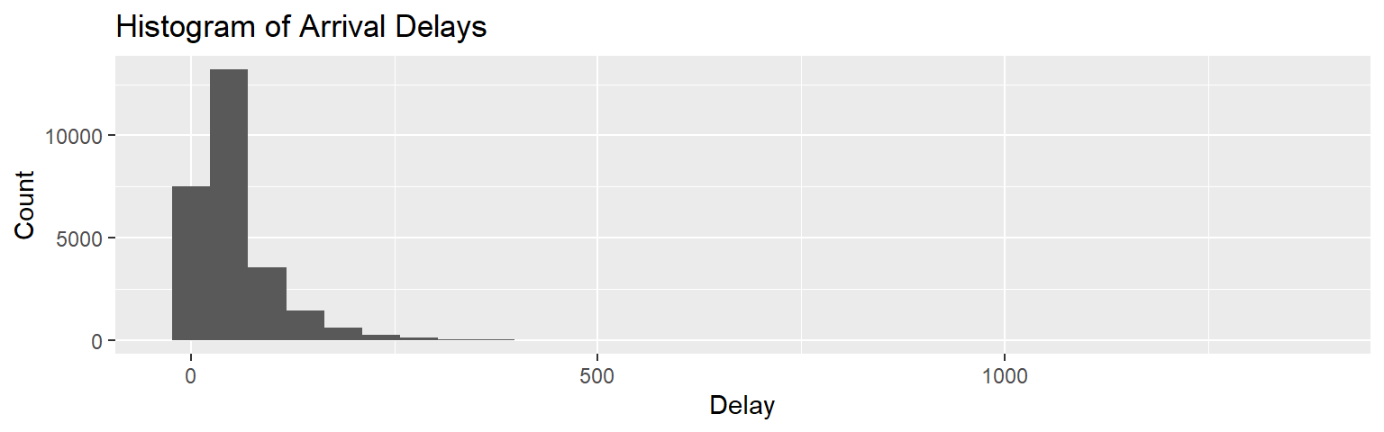
We begin our EDA by looking at the distribution of flight delays. Immediately, we notice that our distribution is not at all symmetric, and thus some kind of data transformation will be required. For our purposes, we will use the log transformation, offsetting our data by \(+15\) within it to get rid of any negative values. All in all, our transformed arrival delay will look like the following:

\[Y_i^*=\log(Y_i+15)\]

After transformation, our data will look like the following. Additionally, we have included Q-Q plots before and after transformation.

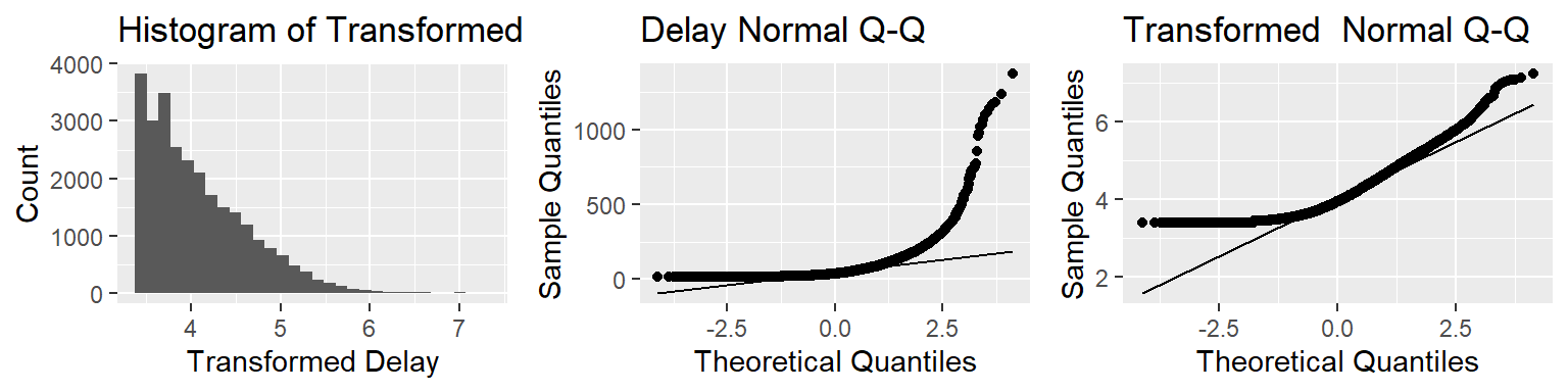
While our data is still not perfectly symmetric, this transformation helps somewhat, and thus we will proceed with our analysis using exclusively transformed delays. We also made a point of looking at some of our bivariate distributions, of which we decided to highlight airline, month, and day Note that month and day are viewed as factor variables, as viewing them as a strictly continuous variable does not allow for variation outside of just an increasing number.

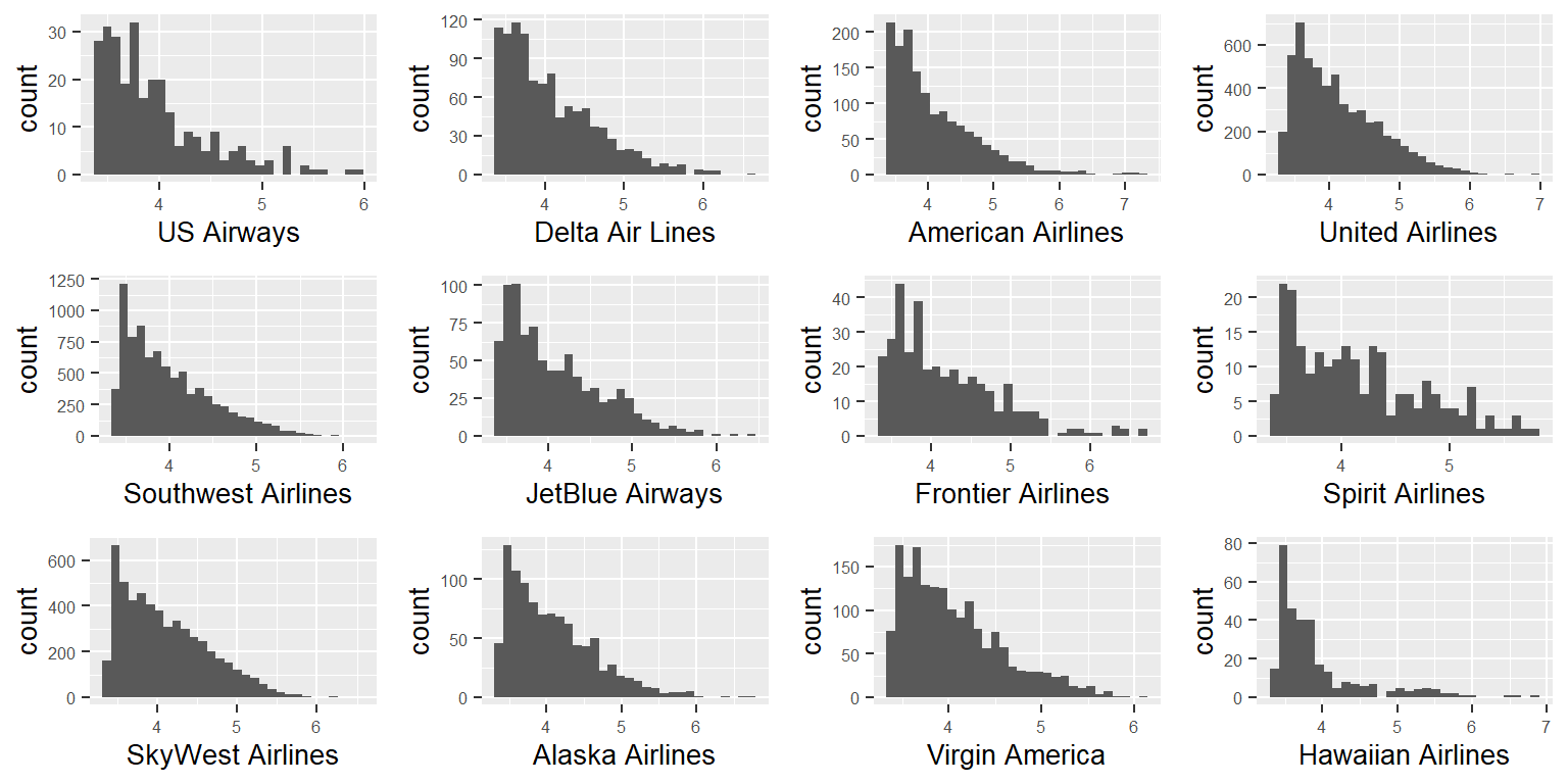
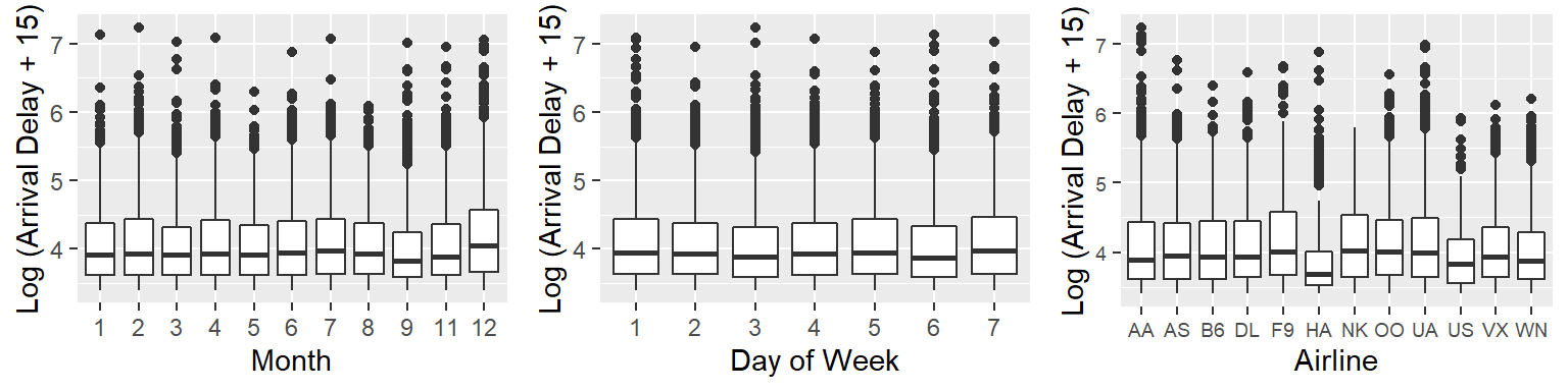
The following major airline carriers operated in 2015 from SFO, OAK, and SJC: US Airways (US), Delta Airlines (DL), American Airlines (AA), United Airlines (UA), Southwest Airlines (WN), JetBlue Airways (B6), Frontier Airlines (F9), Spirit Airlines (NK), Skywest Airlines (OO), Alaska Airlines (AS), Virgin America (VX), and Hawaiian Airlines (HA). Looking at each of the plots for their bivariate distribution with arrival delays, we can note that there seems to be some variation. Specifically, the boxplots reveal to us that HA (Hawaiian Airlines) seems to have far fewer delays on average than other airlines, with most other airlines looking fairly similar in terms of mean and spread. As for Day and Month, most of the days are fairly close in mean, except for December, which seems to have far more average delay than the other months. All in all, it seems worth including these variables in our model to better analyze these differences.

Finally, we can look at a subset of January to attempt to see the difference that time and day may have on flight delays. Looking at the figure above, we notice both peaks at certain times, as well as peaks on certain days (the 6th, the 11th, etc). This further motivates using scheduled departure as a variable in our model.

V. Model Selection

The variables that we will be including in our model selection are Month, Day, Day of the week, Airline, Origin, Destination, Distance, Scheduled Departure, and Scheduled Time (Total Trip Duration). Among them, Month, Day of Week, Airline, Origin, and Destination will all be treated as categorical variables (factors), creating a large number of dummy variables. From the exploratory data analysis done in the last section, we can determine it is unlikely that all of these variables will be of significance to our predictive model, therefore, we decided to conduct some forms of variable pruning.

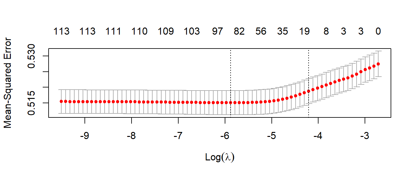
VI. Results

Diagnostics

After using our LASSO regression for model selection, we fit an ordinary least squares regression (OLS) with only the variables with non-zero coefficients in the best model. Generally, refitting using no penalty after having done variable selection via the LASSO is considered “cheating” since you have already looked at the data and the resulting p-values and confidence intervals are not valid in the usual sense. This particular problem is discussed in the published research paper, “In defense of the Indefensible: A Very Naive approach to high-dimensional inference”, The authors conclude that given a large enough dataset and that our explanatory variables are deterministic, “peeking twice” at the data is acceptable. Thus, due to the composition of our design matrix, we can justify this design choice. LASSO, by construction, produces biased estimates for the coefficients, so we would like an unbiased estimate to have better accuracy and better interpretability in our final model. The scale of the delay time is extremely small in respect to the actual flight time, implying our margin for error is small. Flight times in hours yield regression coefficients of minutes or less. Even small bias introduced to the coefficients of our model may endanger the already limited interpretability of our coefficients.

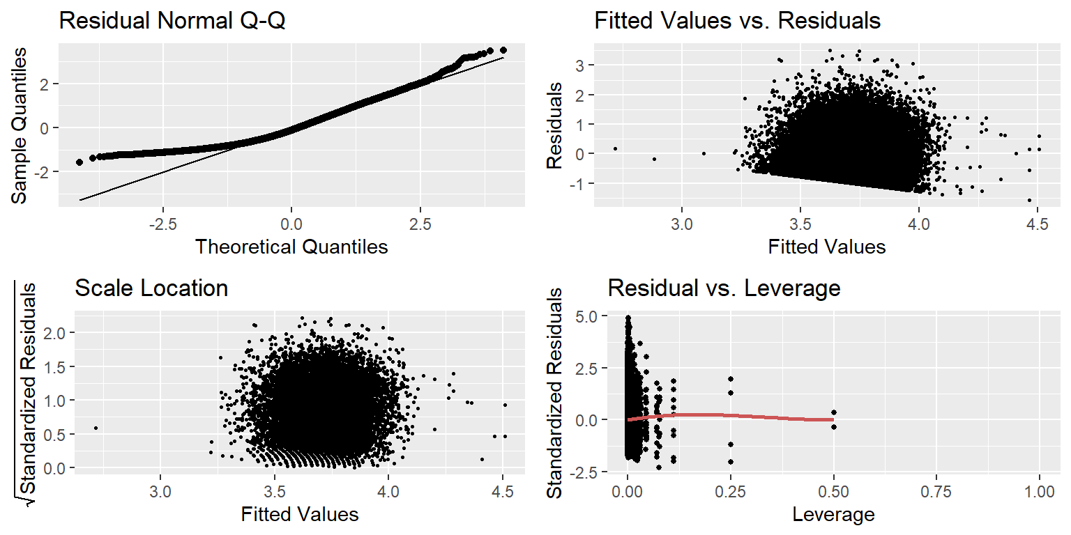
Looking at the figure above, we note the following. First, our plot reveals a significantly non-normal appearing distribution for our residuals. This would be problematic in the case that we wanted to perform inference on our coefficients, but given that we care singularly about prediction, this will not be a problem. Our plot reveals another problem. On the bottom left-hand corner of our model, we observe what seems to be a lower bound on our residuals that slopes down as our fitted values increase. This is likely due to an effective lower bound on Flight Delays. While there is technically no limit to how early our variables can be, there is no flight that arrives earlier than 15 min ahead of schedule, while many flights are significantly later than that. Again, while this would likely be a problem for inference, we are attempting prediction with our model, so it is not much of a concern. The plot shows no discernible trend in our standardized residuals, demonstrating relative homoscedasticity in the distribution of our data points. Finally, while there do seem to be a few points of higher leverage in the plot, we find no values with a Cook’s Distance of greater than \(0.5\), indicating that there do not seem to be any large outliers in our data. Hence, we will not modify our data and proceed to fit and interpret our model as it stands.

VII. Prediction

In our data processing phase, we made a point of setting aside a portion of our data to test our model’s predictive power. We can use this set, which includes \(8,977\) flights, to attempt to analyze the efficacy of our model. We can do this visually and by comparing the RMSE for both our test and training set. For our training data, we obtain an RMSE of \(\approx 0.6712\) and for our test data, we obtain a fairly similar number \(\approx 0.655\). While these values are relatively close to each other and may seem small, it is worth noting that this is in log scale, and these values of RMSE are quite large on a logarithmic scale. This observation is confirmed upon further visual analysis, which gives us the following visualization.

Looking at the above graph, we do note a positive relationship between our actual transformed values and our predicted transformed values, but it is not nearly 1 to 1. More specifically, our model seems to have a great deal of difficulty predicting with higher delay.

VIII. Discussion

Reflecting on the diagnostics and prediction section above, it is clear that our model suffers from some severe limitations. To begin, our model’s residuals are not at all normally distributed and possess both a light left-hand tail and a heavy right-hand tail, even after performing a log transformation. This limits our abilities to form normal confidence intervals from our model, thus limiting our abilities to perform inference. Outside of that, we also run into problems with performing prediction analysis using our model. Our model has an adjusted \(R^2\) of \(\approx 0.028\), implying that only a small portion of the variation in flight delays is accounted for in our data. Moreover, both our test and training data possess fairly large RMSE, indicating a fairly large deviation between what our model predicts and what we see in the data.

All of this together means that our model is not well suited to predict flight delays. While this may seem disheartening after performing all of this analysis, it does give future research into this topic a leg up, as we have established that the variables we analyzed are not predictive of flight delays. Other variables not included with our data may aid with this process, including weather, the number of passengers booked for the flight, the model of the plane, the age of the plane, the price of the flight, and so on. Additionally, other models could likely be explored as well, including models that allow for more interaction between variables or even a multinomial or logistic model that would attempt to predict a degree of lateness, rather than a specific minute count.

IX. Conclusion

Unfortunately, the predicting and inferential power of our model yielded limited results. The scale of predicting flight delays given information about origin airports, airlines, scheduled arrival times, and flight distances explains little of the variation in overall flight delays. Our findings suggest that our model could improve by introducing additional variables not present in our dataset. It is likely that factors such as the weather forecast for the time of the flight in both the departure and destination airports greatly influence the likelihood of a flight delay more so than most of the static variables in our model.

Additionally, fitting a linear regression may not have been the most appropriate application for answering the research question. We saw in our exploratory data analysis that the distribution of flight delays even after taking a log transformation is highly right-skewed. Unfortunately, this suggests that our model would not be able to account for the underlying nonlinearities. Moving forward it may be helpful to stratify the outcome variable into groups and predict the probabilities of on-time arrival, light delay, or heavy delay in a multinomial logistic regression model or through a nested regression model. It may be also helpful to analyze the nonlinearities in flight delays through other nonlinear methods such as polynomial regressions and regression splines. These models may be better equipped to handle the degree of heterogeneity present in our data.

X. References

Zhao, Sen, et al. “In Defense of the Indefensible: A Very Naïve Approach to High-Dimensional Inference.” Statistical Science, vol. 36, no. 4, 2021, https://doi.org/10.1214/20-sts815.

Fox, John. Applied Regression Analysis and Generalized Linear Models. : SAGE Publications, 2008.

US Department of Transportation. (2017, February 9). 2015 Flight Delays and Cancellations (Version 1) [Dataset]. US Department of Transportation. https://www.kaggle.com/usdot/flight-delays

XI. Appendix: All code for this report

knitr::opts_chunk$set(echo = TRUE)
library(glmnet)
library(dplyr)
library(Rcpp)
library(caret)
library(ggplot2)
library(MASS)
library(gridExtra)
library(lindia)
library(latex2exp)
library(lubridate)
set.seed(69)
flights <- na.omit(read.csv("Bay_flights.csv"))
regressors <- c("ARRIVAL_DELAY", "MONTH", "DAY_OF_WEEK", "AIRLINE", 
                "ORIGIN_AIRPORT", "DESTINATION_AIRPORT", 
                "SCHEDULED_DEPARTURE", "DISTANCE")

month_graph <- flights$MONTH

day_graph <- flights$DAY_OF_WEEK

airline_graph <- flights$AIRLINE

destination_graph <- flights$DESTINATION_AIRPORT

flights$MONTH <- as.factor(flights$MONTH)

flights$DAY_OF_WEEK <- as.factor(flights$DAY_OF_WEEK)

dummy <- dummyVars(" ~ .", data = flights[,regressors])

final_df <- data.frame(predict(dummy, newdata=flights[,regressors]))
smp_size <- floor(0.6*nrow(flights))

train_ind <- sample(seq_len(nrow(final_df)), size = smp_size)

train_flights <- final_df[train_ind,]

test_flights <- final_df[-train_ind,]
#Include un-factored versions for graphing
final_df$month_graph <- month_graph

final_df$day_graph <- day_graph

final_df$airline_graph <- airline_graph

final_df$destination_graph <- destination_graph

train_flights_graph <- final_df[train_ind,]

test_flights_graph <- final_df[-train_ind,]
ggplot(data = train_flights_graph) +
  geom_histogram(aes(x = ARRIVAL_DELAY)) +
  labs(title = "Histogram of Arrival Delays", x = "Delay", y = "Count")

## `stat_bin()` using `bins = 30`. Pick better value with `binwidth`.

transformedhist <- ggplot(data = train_flights_graph) +
  geom_histogram(aes(x = log(ARRIVAL_DELAY+15)) ) +
  labs(title = "Histogram of Transformed Arrival Delays", x = "Transformed Delay", y = "Count")

delayqq <- ggplot(data = NULL) +
  stat_qq(aes(sample = train_flights_graph$ARRIVAL_DELAY)) +
  stat_qq_line(aes(sample = train_flights_graph$ARRIVAL_DELAY)) +
  labs(title = "Delay Normal Q-Q",
       x = "Theoretical Quantiles", y = "Sample Quantiles")

transformedqq <- ggplot(data = NULL) +
  stat_qq(aes(sample = log(train_flights_graph$ARRIVAL_DELAY+15))) +
  stat_qq_line(aes(sample = log(train_flights_graph$ARRIVAL_DELAY+15))) +
  labs(title = "Transformed  Normal Q-Q",
       x = "Theoretical Quantiles", y = "Sample Quantiles")

grid.arrange(transformedhist, delayqq, transformedqq, ncol = 3)

## `stat_bin()` using `bins = 30`. Pick better value with `binwidth`.

#Comparing Airlines
US <- ggplot(data = train_flights_graph[train_flights_graph$airline_graph == "US" ,]) + 
  geom_histogram(aes(x = log(ARRIVAL_DELAY + 15))) +
  xlab("US Airways") +
  theme(axis.text=element_text(size=6),
        axis.title=element_text(size=10))

DL <- ggplot(data = train_flights_graph[train_flights_graph$airline_graph == "DL" ,]) + 
  geom_histogram(aes(x = log(ARRIVAL_DELAY + 15))) +
  xlab("Delta Air Lines") +
  theme(axis.text=element_text(size=6), 
        axis.title=element_text(size=10))

AA <- ggplot(data = train_flights_graph[train_flights_graph$airline_graph == "AA" ,]) + 
  geom_histogram(aes(x = log(ARRIVAL_DELAY + 15))) +
  xlab("American Airlines") +
  theme(axis.text=element_text(size=6),
        axis.title=element_text(size=10))

UA <- ggplot(data = train_flights_graph[train_flights_graph$airline_graph == "UA" ,]) + 
  geom_histogram(aes(x = log(ARRIVAL_DELAY + 15))) +
  xlab("United Airlines") +
  theme(axis.text=element_text(size=6),
        axis.title=element_text(size=10))

WN <- ggplot(data = train_flights_graph[train_flights_graph$airline_graph == "WN" ,]) + 
  geom_histogram(aes(x = log(ARRIVAL_DELAY + 15))) +
  xlab("Southwest Airlines") +
  theme(axis.text=element_text(size=6),
        axis.title=element_text(size=10))

B6 <- ggplot(data = train_flights_graph[train_flights_graph$airline_graph == "B6" ,]) + 
  geom_histogram(aes(x = log(ARRIVAL_DELAY + 15))) +
  xlab("JetBlue Airways") +
  theme(axis.text=element_text(size=6),
        axis.title=element_text(size=10))

F9 <- ggplot(data = train_flights_graph[train_flights_graph$airline_graph == "F9" ,]) + 
  geom_histogram(aes(x = log(ARRIVAL_DELAY + 15))) +
  xlab("Frontier Airlines") +
  theme(axis.text=element_text(size=6),
        axis.title=element_text(size=10))

NK <- ggplot(data = train_flights_graph[train_flights_graph$airline_graph == "NK" ,]) + 
  geom_histogram(aes(x = log(ARRIVAL_DELAY + 15))) +
  xlab("Spirit Airlines")+
  theme(axis.text=element_text(size=6),
        axis.title=element_text(size=10))

OO <- ggplot(data = train_flights_graph[train_flights_graph$airline_graph == "OO" ,]) + 
  geom_histogram(aes(x = log(ARRIVAL_DELAY + 15))) +
  xlab("SkyWest Airlines") +
  theme(axis.text=element_text(size=6),
        axis.title=element_text(size=10))

AS <- ggplot(data = train_flights_graph[train_flights_graph$airline_graph == "AS" ,]) + 
  geom_histogram(aes(x = log(ARRIVAL_DELAY + 15))) +
  xlab("Alaska Airlines") +
  theme(axis.text=element_text(size=6),
        axis.title=element_text(size=10))

VX <- ggplot(data = train_flights_graph[train_flights_graph$airline_graph == "VX" ,]) + 
  geom_histogram(aes(x = log(ARRIVAL_DELAY + 15))) +
  xlab("Virgin America") +
  theme(axis.text=element_text(size=6),
        axis.title=element_text(size=10))

HA <- ggplot(data = train_flights_graph[train_flights_graph$airline_graph == "HA" ,]) + 
  geom_histogram(aes(x = log(ARRIVAL_DELAY + 15))) +
  xlab("Hawaiian Airlines") +
  theme(axis.text=element_text(size=6),
        axis.title=element_text(size=10))

grid.arrange(US, DL, AA, UA, WN, B6, F9, NK, OO, AS, VX, HA, ncol = 4)

## `stat_bin()` using `bins = 30`. Pick better value with `binwidth`.
## `stat_bin()` using `bins = 30`. Pick better value with `binwidth`.
## `stat_bin()` using `bins = 30`. Pick better value with `binwidth`.
## `stat_bin()` using `bins = 30`. Pick better value with `binwidth`.
## `stat_bin()` using `bins = 30`. Pick better value with `binwidth`.
## `stat_bin()` using `bins = 30`. Pick better value with `binwidth`.
## `stat_bin()` using `bins = 30`. Pick better value with `binwidth`.
## `stat_bin()` using `bins = 30`. Pick better value with `binwidth`.
## `stat_bin()` using `bins = 30`. Pick better value with `binwidth`.
## `stat_bin()` using `bins = 30`. Pick better value with `binwidth`.
## `stat_bin()` using `bins = 30`. Pick better value with `binwidth`.
## `stat_bin()` using `bins = 30`. Pick better value with `binwidth`.

#Boxplots
months <- ggplot(data = train_flights_graph) + 
  geom_boxplot(aes(y = log(ARRIVAL_DELAY + 15), 
                   x = as.factor(month_graph)) ) + 
  xlab("Month") + ylab("Log (Arrival Delay + 15)")

days <- ggplot(data = train_flights_graph) + 
  geom_boxplot(aes(y = log(ARRIVAL_DELAY + 15), x = as.factor(day_graph)) ) + 
  xlab("Day of Week") + ylab("Log (Arrival Delay + 15)")

airlines <- ggplot(data = train_flights_graph) + 
  geom_boxplot(aes(y = log(ARRIVAL_DELAY + 15), x = as.factor(airline_graph))) + 
  xlab("Airline") + ylab("Log (Arrival Delay + 15)") +
  theme(axis.text=element_text(size=7),
        axis.title=element_text(size=11))

grid.arrange(months, days, airlines, ncol = 3)

#Scatterplot Time

#generate noise
noise_1 <- runif(nrow(train_flights_graph), min = -25, max = 25)
noise_2 <- runif(nrow(train_flights_graph), min = -10, max = 10)

ggplot(data = train_flights_graph, 
       aes(y = log(ARRIVAL_DELAY + 15), x = DISTANCE + noise_1)) + 
  geom_point(size = 0.25) + 
  geom_smooth(method = "lm", 
              formula = y~x)

ggplot(data = train_flights_graph, 
       aes(y = log(ARRIVAL_DELAY + 15), x = SCHEDULED_DEPARTURE + noise_1)) + 
  geom_point(size = 0.25) + 
  geom_smooth(method = "lm", formula = y ~x)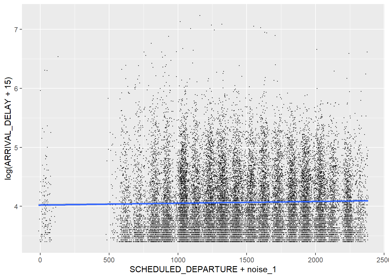

ggplot(data = train_flights_graph, 
       aes(y = log(ARRIVAL_DELAY + 15), 
           x = SCHEDULED_DEPARTURE + noise_1, color = as.factor(month_graph))) + 
  geom_point(size = 0.5) + 
  geom_smooth(method = "lm", formula = y ~x, se = FALSE)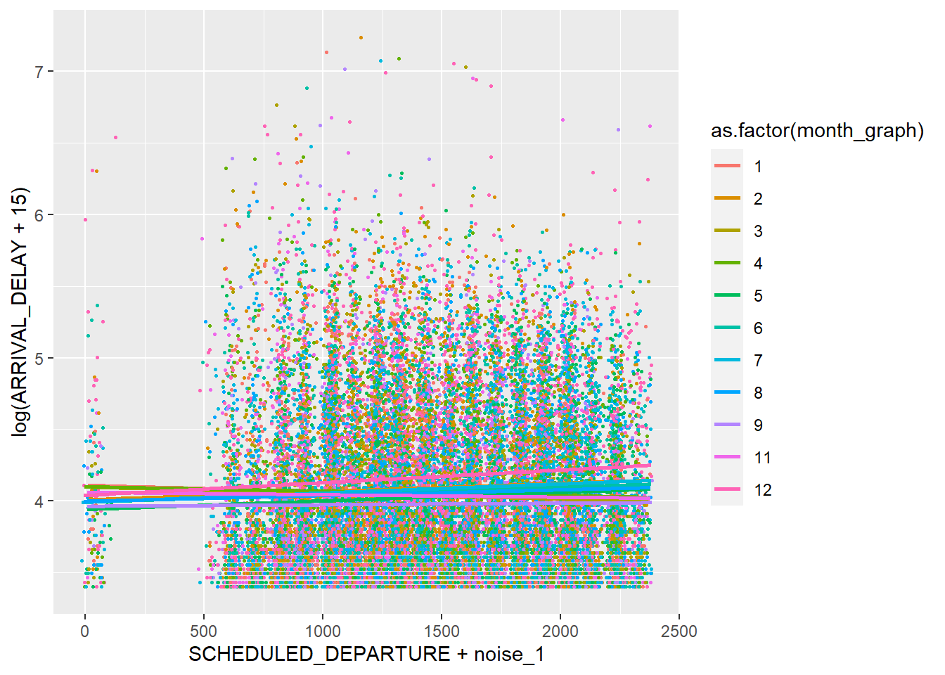

#Temporal Variability of Delay
select_flights <-  flights[, c("ARRIVAL_DELAY", "YEAR", "MONTH", "DAY", "SCHEDULED_DEPARTURE")]


select_flights$date <- make_datetime(year = select_flights$YEAR, 
                                  month = select_flights$MONTH, 
                                  day = select_flights$DAY, 
                                  hour = select_flights$SCHEDULED_DEPARTURE %/% 100,
                                  min = select_flights$SCHEDULED_DEPARTURE %% 100)


ggplot(data = select_flights[select_flights$MONTH == 1 & 
                               select_flights$DAY >= 1 & 
                               select_flights$DAY <=15,  ], 
       aes(x = date, y = log(ARRIVAL_DELAY+15))) + 
    geom_line() + 
    ylab("Log Arrival Delay") + xlab("Date") +
    scale_x_datetime(breaks = scales::breaks_pretty(14)) +
    theme(axis.text=element_text(size=7),
      axis.title=element_text(size=11))

#Cross Validation to find optimal lambda
cv_model <- cv.glmnet(x = as.matrix(train_flights[-1]), y = log(train_flights[[1]]), alpha = 1)
#using our optimized lambda from before to create a best lasso model
best_lambda <- cv_model$lambda.min
best_model <- glmnet(x = as.matrix(train_flights[-1]), y = log(train_flights[[1]] + 15), alpha = 1, lambda = best_lambda)

#removing rows that are non-zero to extract our coefficients
final_regressors <- rownames(coef(best_model))[coef(best_model)[ ,1] != 0][-1][-11]
#creating a formula for using with lm
regressors <- paste(final_regressors, collapse = " + ")

lasso_formula <- as.formula(paste("log(ARRIVAL_DELAY) ~ ", regressors, sep = ""))
#lm with reduced set of coefficients
final_model <-lm(data = train_flights, formula = lasso_formula)

summary(final_model)

## 
## Call:
## lm(formula = lasso_formula, data = train_flights)
## 
## Residuals:
##     Min      1Q  Median      3Q     Max 
## -1.5728 -0.5775 -0.1139  0.4786  3.4974 
## 
## Coefficients:
##                          Estimate Std. Error t value Pr(>|t|)    
## (Intercept)             3.595e+00  3.126e-02 115.011  < 2e-16 ***
## MONTH.1                -2.604e-02  1.785e-02  -1.459 0.144689    
## MONTH.2                 2.223e-02  1.880e-02   1.182 0.237156    
## MONTH.3                -3.833e-02  1.856e-02  -2.065 0.038936 *  
## MONTH.5                -3.980e-02  1.749e-02  -2.275 0.022930 *  
## MONTH.6                 1.831e-02  1.730e-02   1.058 0.289892    
## MONTH.7                 5.127e-02  1.692e-02   3.030 0.002451 ** 
## MONTH.9                -1.021e-01  2.044e-02  -4.996 5.90e-07 ***
## MONTH.11               -2.889e-02  1.939e-02  -1.490 0.136262    
## MONTH.12                1.388e-01  1.639e-02   8.466  < 2e-16 ***
## DAY_OF_WEEK.1           4.326e-02  1.329e-02   3.254 0.001141 ** 
## DAY_OF_WEEK.3          -4.836e-02  1.460e-02  -3.312 0.000926 ***
## DAY_OF_WEEK.5           4.770e-02  1.356e-02   3.517 0.000437 ***
## DAY_OF_WEEK.6          -3.000e-02  1.745e-02  -1.719 0.085545 .  
## DAY_OF_WEEK.7           6.589e-02  1.360e-02   4.845 1.27e-06 ***
## AIRLINEB6              -6.584e-02  3.019e-02  -2.181 0.029180 *  
## AIRLINEF9               8.589e-02  4.278e-02   2.008 0.044703 *  
## AIRLINEHA              -1.415e-01  4.841e-02  -2.923 0.003472 ** 
## AIRLINENK               1.641e-01  5.285e-02   3.104 0.001912 ** 
## AIRLINEOO              -4.990e-03  1.842e-02  -0.271 0.786499    
## AIRLINEUA               3.238e-02  1.759e-02   1.841 0.065593 .  
## AIRLINEUS              -3.110e-02  5.200e-02  -0.598 0.549727    
## AIRLINEVX              -8.399e-02  2.250e-02  -3.732 0.000190 ***
## AIRLINEWN              -8.093e-02  1.898e-02  -4.264 2.01e-05 ***
## ORIGIN_AIRPORTOAK      -1.330e-02  1.570e-02  -0.847 0.397097    
## ORIGIN_AIRPORTSFO       8.776e-02  1.519e-02   5.776 7.76e-09 ***
## DESTINATION_AIRPORTABQ -1.078e-01  6.100e-02  -1.768 0.077074 .  
## DESTINATION_AIRPORTASE  1.263e-01  1.237e-01   1.021 0.307372    
## DESTINATION_AIRPORTATL -1.727e-01  4.620e-02  -3.739 0.000185 ***
## DESTINATION_AIRPORTBNA -2.026e-01  1.537e-01  -1.318 0.187517    
## DESTINATION_AIRPORTBOS  3.824e-02  3.833e-02   0.998 0.318429    
## DESTINATION_AIRPORTBUR  3.588e-02  2.858e-02   1.256 0.209255    
## DESTINATION_AIRPORTBWI -9.045e-02  7.825e-02  -1.156 0.247724    
## DESTINATION_AIRPORTCLT -2.910e-01  7.051e-02  -4.127 3.69e-05 ***
## DESTINATION_AIRPORTCMH  7.750e-01  1.995e-01   3.884 0.000103 ***
## DESTINATION_AIRPORTCOS -7.178e-01  7.163e-01  -1.002 0.316293    
## DESTINATION_AIRPORTDAL -5.263e-02  4.279e-02  -1.230 0.218675    
## DESTINATION_AIRPORTDCA -1.871e-01  8.373e-02  -2.235 0.025443 *  
## DESTINATION_AIRPORTDEN  1.459e-02  2.534e-02   0.576 0.564730    
## DESTINATION_AIRPORTDFW  4.368e-02  3.025e-02   1.444 0.148695    
## DESTINATION_AIRPORTDTW -3.341e-01  8.175e-02  -4.087 4.38e-05 ***
## DESTINATION_AIRPORTFAT  9.160e-02  6.718e-02   1.364 0.172687    
## DESTINATION_AIRPORTHDN -9.640e-01  5.067e-01  -1.902 0.057120 .  
## DESTINATION_AIRPORTHOU -1.153e-01  8.637e-02  -1.335 0.181764    
## DESTINATION_AIRPORTIAH -6.107e-02  3.227e-02  -1.892 0.058449 .  
## DESTINATION_AIRPORTIND  2.435e-01  1.236e-01   1.970 0.048800 *  
## DESTINATION_AIRPORTJAC  1.525e-01  1.127e-01   1.353 0.176016    
## DESTINATION_AIRPORTJFK  1.112e-01  2.934e-02   3.790 0.000151 ***
## DESTINATION_AIRPORTLAX -2.623e-02  1.653e-02  -1.587 0.112518    
## DESTINATION_AIRPORTMCI -9.683e-02  6.684e-02  -1.449 0.147447    
## DESTINATION_AIRPORTMCO -8.428e-02  7.844e-02  -1.074 0.282649    
## DESTINATION_AIRPORTMFR -8.759e-02  5.491e-02  -1.595 0.110711    
## DESTINATION_AIRPORTMMH  1.640e-01  1.920e-01   0.854 0.392989    
## DESTINATION_AIRPORTMRY  1.074e-01  8.531e-02   1.258 0.208254    
## DESTINATION_AIRPORTMSO  3.334e-01  2.392e-01   1.394 0.163432    
## DESTINATION_AIRPORTMSP -1.629e-01  4.846e-02  -3.361 0.000778 ***
## DESTINATION_AIRPORTOGG -3.647e-02  4.510e-02  -0.809 0.418712    
## DESTINATION_AIRPORTONT  3.396e-02  3.035e-02   1.119 0.263154    
## DESTINATION_AIRPORTORD -4.643e-02  2.607e-02  -1.781 0.074920 .  
## DESTINATION_AIRPORTOTH  1.211e-01  9.944e-02   1.217 0.223431    
## DESTINATION_AIRPORTPDX  1.764e-02  2.673e-02   0.660 0.509216    
## DESTINATION_AIRPORTPHL -1.372e-01  5.480e-02  -2.504 0.012301 *  
## DESTINATION_AIRPORTPIT -2.047e-01  1.503e-01  -1.362 0.173333    
## DESTINATION_AIRPORTPSC  2.124e-01  1.127e-01   1.886 0.059372 .  
## DESTINATION_AIRPORTPSP  4.915e-02  4.515e-02   1.089 0.276327    
## DESTINATION_AIRPORTRDU  8.457e-02  9.616e-02   0.880 0.379118    
## DESTINATION_AIRPORTRNO  9.940e-02  5.522e-02   1.800 0.071839 .  
## DESTINATION_AIRPORTSAN  2.025e-02  2.174e-02   0.932 0.351558    
## DESTINATION_AIRPORTSBA  5.243e-02  4.990e-02   1.051 0.293418    
## DESTINATION_AIRPORTSEA -2.795e-02  2.167e-02  -1.290 0.197024    
## DESTINATION_AIRPORTSLC  4.477e-02  2.978e-02   1.503 0.132781    
## DESTINATION_AIRPORTSMF  6.143e-02  5.556e-02   1.106 0.268822    
## DESTINATION_AIRPORTSNA -1.190e-01  2.713e-02  -4.386 1.16e-05 ***
## DESTINATION_AIRPORTSUN -3.392e-01  1.273e-01  -2.664 0.007728 ** 
## DESTINATION_AIRPORTXNA  3.448e-01  3.585e-01   0.962 0.336137    
## SCHEDULED_DEPARTURE     5.147e-05  1.012e-05   5.085 3.69e-07 ***
## DISTANCE               -9.587e-06  1.055e-05  -0.909 0.363518    
## ---
## Signif. codes:  0 '***' 0.001 '**' 0.01 '*' 0.05 '.' 0.1 ' ' 1
## 
## Residual standard error: 0.716 on 26854 degrees of freedom
## Multiple R-squared:  0.03102,    Adjusted R-squared:  0.02828 
## F-statistic: 11.31 on 76 and 26854 DF,  p-value: < 2.2e-16

plot(cv_model)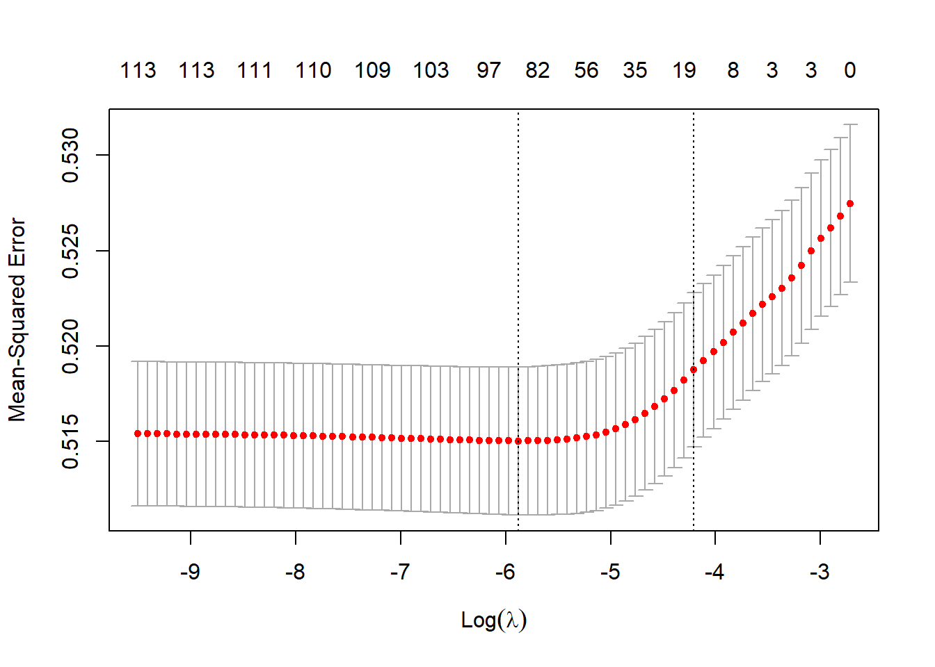

qqresid <- ggplot(data = NULL) + stat_qq(aes(sample = final_model$residuals)) +
  stat_qq_line(aes(sample = final_model$residuals)) +
  labs(title = "Residual Normal Q-Q",
       x = "Theoretical Quantiles", y = "Sample Quantiles")

fittedresid <- ggplot(final_model) + 
  geom_point(aes(x=.fitted, y=.resid), size = 0.5) +
  labs(title = "Fitted Values vs. Residuals", x = "Fitted Values",
       y = "Residuals")

scalelocation <- ggplot(final_model) + 
  geom_point(aes(x=.fitted, y=sqrt(rstandard(final_model))), size = 0.5) + 
  labs(title = "Scale Location", x = "Fitted Values", 
       y = TeX("$$\\sqrt{Standardized Residuals}$$"))

leverage <- gg_resleverage(final_model, method = "loess",
                           se = FALSE, scale.factor = 1)

grid.arrange(qqresid, fittedresid, scalelocation, leverage, ncol = 2)

## Warning in sqrt(rstandard(final_model)): NaNs produced

## Warning in sqrt(rstandard(final_model)): NaNs produced

## Warning: Removed 14887 rows containing missing values (geom_point).

## `geom_smooth()` using formula 'y ~ x'

## Warning: Removed 1 rows containing non-finite values (stat_smooth).

## Warning: Removed 1 rows containing missing values (geom_point).

sum(cooks.distance(final_model) >= 0.5)

## [1] NA

predictions <- predict(final_model, newdata = test_flights)

training_predictions <- predict(final_model, newdata = train_flights)

RMSEtest <- sqrt(mean(((log(test_flights[,1]+15) - predictions)^2)))

RMSEtraining <- sqrt(mean(((log(train_flights[,1]+15) - predictions)^2)))

## Warning in log(train_flights[, 1] + 15) - predictions: longer object length is
## not a multiple of shorter object length

prediction_df <- data.frame(log(test_flights[,1]+15) , predictions)

colnames(prediction_df) <- c("Actual", "Predicted")
ggplot(data = prediction_df, aes(x = Actual, y = Predicted)) + geom_point() + 
  geom_smooth(method = "lm", se = FALSE) +
  labs( x = "Actual Transformed Delay",
       y = "Predicted Transformed Delay")

## `geom_smooth()` using formula 'y ~ x'